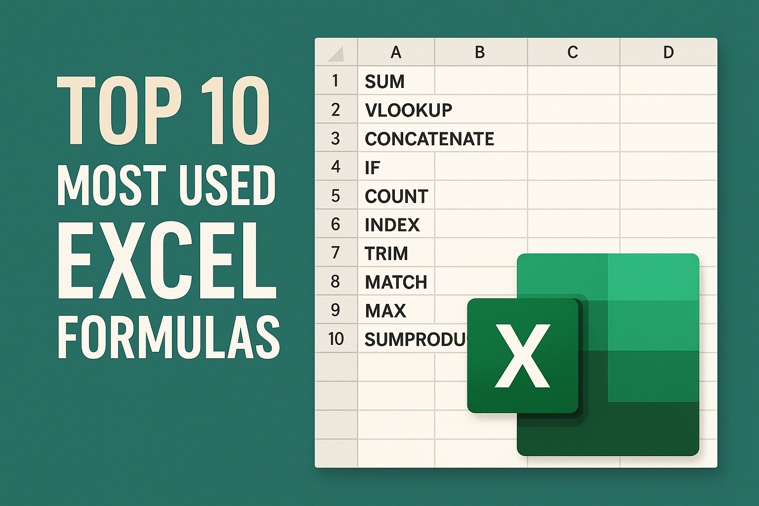
Top 10 Most Used Excel Formulas — With Real, Copy‑Paste Examples

Stop skimming lists that barely help. This guide is designed for action: each formula includes a scenario, a tested snippet, a pitfall to avoid, and a short exercise so you can confirm you actually learned it.

Tip: Try the examples in a blank sheet as you read. Most snippets work as‑is.

1) SUM — Fast, Flexible Totals

🎯 Scenario: Total monthly sales in B2:B13.

• Snippet: =SUM(B2:B13)
• Also works (non‑adjacent ranges): =SUM(B2:B13, D2:D13)

Pitfall: Text that “looks like” numbers won’t sum. Wrap the range with VALUE() or fix the import.

Mini exercise: Create numbers in B2:B6 and confirm your total matches a manual check.

2) AVERAGE / MEDIAN — Understand the Middle

🎯 Scenario: Teacher grading in C2:C31.

• Mean: =AVERAGE(C2:C31)
• Robust to outliers: =MEDIAN(C2:C31)

Pitfall: Empty cells are ignored, zeros are not. Use AVERAGEIF(C2:C31,">=") to ignore blanks that are actually empty strings.

Mini exercise: Add a single extreme value and compare AVERAGE vs MEDIAN.

3) COUNT / COUNTA — How Many Values?

• Numbers only: =COUNT(D2:D100)
• Anything non‑blank: =COUNTA(D2:D100)

Pitfall: Spaces count as text. Use TRIM() or clean your data before using COUNTA.

4) IF / IFS — Add Logic Without Code

🎯 Scenario: Flag invoices as overdue if days > 30.

• Simple: =IF(E2>30, "Overdue", "On Time")
• Multiple conditions (clearer than nested IFs):

= =IFS(E2>60,"Critical", E2>30,"Overdue", E2>0,"Pending", TRUE,"On Time") =

Pitfall: Order matters in IFS. First match wins.

Mini exercise: Add a Paid status that overrides everything else with IF(Paid="Yes","Paid", yourIFS).

5) XLOOKUP (or VLOOKUP) — Find Things Reliably

Prefer XLOOKUP over VLOOKUP — it works left/right, has exact‑match by default, and returns better errors.

• XLOOKUP: =XLOOKUP("John", A2:A100, C2:C100, "Not found")
• Classic VLOOKUP (if you must): =VLOOKUP("John", A2:C100, 3, FALSE)

Pitfall: With VLOOKUP, the lookup column must be the first column in the table. XLOOKUP has no such limitation.

Mini exercise: Swap the columns and confirm VLOOKUP breaks while XLOOKUP still works.

6) INDEX + MATCH — Power and Flexibility

When XLOOKUP isn’t available, use this dependable duo.

= =INDEX(C2:C100, MATCH("Product X", A2:A100, 0)) =

• Two‑way lookup (row + column):

= =INDEX(C2:G100, MATCH("Product X", A2:A100, 0), MATCH("May", C1:G1, 0)) =

Pitfall: The third argument of MATCH should be 0 for exact match 99% of the time.

7) MIN / MAX — Instant Extremes

= =MIN(H2:H366) =MAX(H2:H366) =

Enhance with conditional formatting to auto‑highlight best/worst days.

8) SUMIF / COUNTIF / AVERAGEIF — Criteria Math

🎯 Scenario: Sales over $100 in E2:E100.

• Total: =SUMIF(E2:E100, ">100")

• Count: =COUNTIF(E2:E100, ">100")

• Average: =AVERAGEIF(E2:E100, ">100")

• Multiple criteria (date range + region):

= =SUMIFS(F2:F100, A2:A100, ">="&DATE(2025,1,1), A2:A100, "<"&DATE(2026,1,1), B2:B100, "North") =

Pitfall: Criteria for dates must be text joined with & as above.

9) TEXT — Beautiful, Useful Formatting

• Dates: =TEXT(A2, "dddd, mmmm d, yyyy")
• Currency with sign: =TEXT(B2, "$#,##0.00")
• IDs: =TEXT(ROW(), "INV-0000") → INV-0001, INV-0002, …

Pitfall: TEXT returns text. If you need numbers later, wrap with VALUE().

10) CONCAT / & / TEXTJOIN — Build Clean Labels

• Quick full name: =A2&" "&B2
• Ignore blanks (best practice): =TEXTJOIN(" ", TRUE, A2, B2, C2)

Pitfall: CONCATENATE() is legacy. Prefer &, CONCAT, or TEXTJOIN.

Putting It Together — A Compact KPI Card

Create a single sentence KPI summary from raw data:

= ="Q"&TEXT(TODAY(),"Q")&" sales were "&TEXT(SUMIFS(Sales,Region,"North",Date,">="&EOMONTH(TODAY(),-3)+1,Date,"<="&EOMONTH(TODAY(),0)),"$#,##0")& " ("&COUNTIFS(Region,"North",Date,">="&EOMONTH(TODAY(),-3)+1,Date,"<="&EOMONTH(TODAY(),0))&" orders), avg "& TEXT(AVERAGEIFS(Sales,Region,"North",Date,">="&EOMONTH(TODAY(),-3)+1,Date,"<="&EOMONTH(TODAY(),0)),"$#,##0") =

This combines TEXT, SUMIFS, COUNTIFS, and AVERAGEIFS into one presentation‑ready sentence.

Quick Checklist (copy to your sheet)

• Exact matches use 0 in MATCH or the default in XLOOKUP
• Date criteria wrapped with text and &
• Watch for numbers stored as text
• Prefer TEXTJOIN over fragile & chains when ignoring blanks
• Test each piece separately if something breaks

If you want a hands‑on way to master these, try the exercises in the app — each mirrors a real business scenario and reinforces the patterns above.